Principal Component Analysis in Aerodynamic Shape Optimisation

When my Kohai asked “why reduce dimensions?”, the Senpai replied back “because it works!”.

This article will highlight the potential use of Principal Component Analysis (or PCA) as a useful tool in aerodynamic shape optimisation related problems. This article is not meant to serve as an introduction to PCA itself, for which a plethora of good articles already exists. The analysis is based on the data obtained in a recent study by Brahmachary and Ogawa 2021, where a multi-point multi-objective optimisation problem for scramjet intake was undertaken.

PCA is a data-driven dimensionality reduction technique. Ever since its inception in 1901, it has seen widespread use in fields such as image compression, classification, face recognition, anomaly detection, etc. The present article will focus on the use of PCA in dimensionality reduction (or data compression) and flowfield (or image) classification, for high-dimensional data obtained from Computational Fluid Dynamics (CFD) based numerical simulations.

It is often seen that aerodynamic shape optimisation (or ASO) problems targets to achieve shapes that either maximise or minimise certain performance measures, e.g., drag/lift coefficient, efficiency, etc. These scalar quantities of interest QoI themselves depend on high-fidelity flowfield data governed by partial differential equations. Consequently, one can envisage a scenario where these unique high-fidelity flowfield data are evaluated as many times as there are unique combinations of decision variables produced by the optimiser.

Decision variables: Vector of input values or parameters which determine the shape of the geometry (or scramjet intake in this case).

For typical optimisation problems with multiple objectives (i.e., multi-objective optimisation MDO) solved using evolutionary algorithms, the final optimal solution is usually more than 1. The set of optimal solutions is referred to as Pareto optimal solution. The evolutionary algorithm based optimisation starts with an initial population of solutions (or geometries) and with MDO generations, this search concludes with a Pareto optimal front. In this process from start to finish, the search algorithm evaluates multiple flowfields and subsequently determines the QoI. Processing such large ensemble of high-fidelity flowfield data is challenging and motivates the use of dimensionality reduction techniques.

Pareto optimal solution: Set of (non-dominated) optimal solutions obtained in a multi-objective optimisation problem.

Flowfield: High-fidelity data that are the discrete solutions to underlying conservation laws. These data often represent the spatial/temporal variation of field variables such as static pressure, density, velocity, temperature, etc.

Dimensionality reduction technique (e.g., PCA) can be utilised to not only compress the high-dimensional data but in the subsequent sections, it will be shown how PCA can be utilised to extract useful information in a lower-dimensional space spanned by the principal components. Particularly, this article will highlight how PCA is used as an image classifier for high-fidelity CFD flowfield data.

The crucial steps involved in PCA can be summarised as follows:

Create the data matrix $\mathbf{X}$ : Every row of this matrix is composed of the nodal values of a field variable(s), e.g., static pressure. There is n number of nodes in a flowfield. Every column of this matrix corresponds to a flowfield m. Consequently, $\mathbf{X} \in \mathbf{R} ^{n \times m}$
Compute the average or mean matrix $\bar{\mathbf{X}}$ such that $\mathbf{\bar{X}} = [1, 1, 1 ... 1]^ \mathrm{'} \frac{1}{n} \sum_{i=1}^{n} \mathbf{X}_{\mathrm{i}}$
Subtract original data matrix from mean matrix to generate the mean-centered data $\mathbf{M} = \mathbf{X} - \bar{\mathbf{X}}$ . This is necessary as computing PCA is sensitive to the variance in the data.
Compute the covariance matrix of $\mathbf{C} = \mathbf{M}^{\mathrm{'}} \mathbf{M}$ . This step enables us to find out highly correlated data existing in our dataset.
Compute eigenvectors $\mathbf{V}$ and eigenvalues $\mathbf{D}$ of the covariance matrix $\mathbf{C}$ . The eigenvectors $\mathbf{V}$ indicate the direction of the most variance. The principal components are then evaluated as $\mathbf{T} = \mathbf{B} \mathbf{V}$ .

The above steps enable us to decompose the input data matrix $\mathbf{X}$ into principal components, which indicate the directions of maximum variance. In $\texttt{MATLAB}$ this can be done by evaluating the Singular Value Decomposition (SVD) of the mean-centered matrix $\mathbf{M}$ as,

$[\mathrm{U, S, V}] = \texttt{svd(M,`econ');}$

where $\texttt{econ}$ refers to economy option of SVD. In $\texttt{Python}$ , this can be done using the following command,

$[\mathrm{U, S, V}] = \texttt{np.linalg.svd}(\mathbf{M})$

It now follows, $\mathbf{T} = \mathbf{M} \mathbf{V} = \mathbf{U} \sum \mathbf{V}^\mathrm{'} \mathbf{V} =\mathbf{U} \sum$

Flowfield reconstruction:

Following the decomposition of the large data-matrix $\mathbf{M}$ , the matrix $\mathbf{U} \in \mathbf{R} ^{n \times m}$ and $\mathbf{V} \in \mathbf{R} ^{n \times m}$ are referred to as left and right singular matrix, respectively whereas the elements of the diagonal matrix $\sum \in \mathbf{R} ^{n \times m}$ are called singular values. The singular values $\sigma_\mathrm{i}$ are non-zero and are ordered from largest to smallest.

Now that we have covered the basics of PCA, we would like to see how useful it is in data compression. As mentioned earlier, the original data matrix $\mathbf{X}$ often contains highly correlated or redundant information, which can be safely neglected. Put in another way, it is possible to reconstruct $\mathbf{X}$ using $r$ columns of $\mathbf{U}$ , $r$ columns of $\mathbf{V}$ and $r \times r$ truncated $\mathbf{U}$ , where $r << m$ , i.e.

$\mathbf{X}_{recon} = \mathbf{U}_r \sum_r \mathbf{V}_r^{'}$

Accuracy of reconstructed $\mathbf{X}$ increases with increasing $r$ . For $r = m$ , one can exactly reconstruct the original flowfield. One way to determine a safe value of $r$ or PCA modes is to plot the singular values $\sigma_l$ or the cumulative sum of the singular values, i.e.,

$\mathrm{Cumulative \ sum} = \frac{\sum_{i=1}^{r}\sigma_i}{\sum_{i=1}^{m}\sigma_i}$

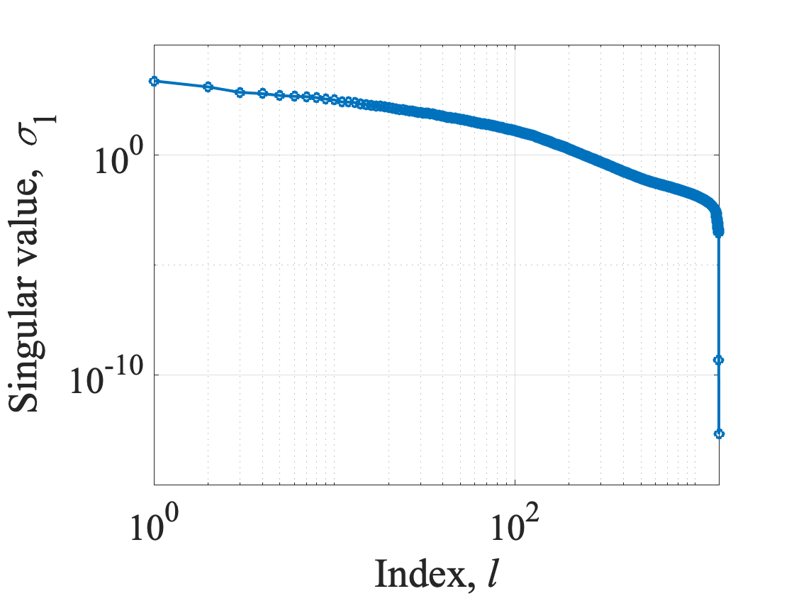
A quick look at the figures above indicates that there is a continuous decrease in $\sigma_l$ however, the trend is not indicative of a rapid fall, signifying that one cannot expect to obtain an accurate representation of $\mathbf{X}$ using only a few PCA modes $r$ . This is evident in the flowfields (any column of $\mathbf{X}$ ) reconstructed using $r$ = 1 (the flowfield depicts the Mach number flowfield distribution inside a scramjet intake which features hypersonic entry).

It is clear that the reconstructed flowfield and the actual flowfield (solutions of Euler equations) are completely different when just 1 PCA mode is used. However, for $r$ = 10, there is a significant improvement in the flowfield reconstruction with the exception of a diffused oblique shock at the entry and inlet exit. More importantly, however, $r$ = 100 results in a significantly accurate flowfield throughout the intake. This shows that using just $r$ = 100 offers a significant data compression when compared to the total number of flowfields, i.e., $m = 1351$

$\texttt{A note of Caution:}$ It must be mentioned here that while such approaches offer tremendous potential in image compression, one must be careful with high-fidelity data obtained from numerical simulations, as they are an outcome of solutions to conservation equations, which is likely to be lost in translation.

Flowfield classification:

PCA offers tremendous potential for image classification and pattern recognition. Given that a lot of data is obtained at the end of MDO, it is impractical to analyse the data as it is, which would require a $m$ dimensional space. Data reduction using PCA offers a potential solution to this problem by significantly reducing the dimensional to a few (e.g., space spanned by the first three principal components). The task of analysing the data becomes more tractable then.

The results from the study performed by Brahmachary and Ogawa 2021 showed that the Pareto optimal front exhibits two broad patterns, as can be observed above in the Mach number flowfield distributions, i.e., some flowfield features a distinct shock whereas others were characterised by diffused compression waves.

The above posed a question – if the higher dimensional data showed signs of distinct pattern, would they exhibit some pattern in a lower-dimensional space with a clear separation or boundary between the solutions in each cluster? To find out, it was necessary to perform PCA on the Pareto optimal solutions, which comprised of 32 unique flowfields.

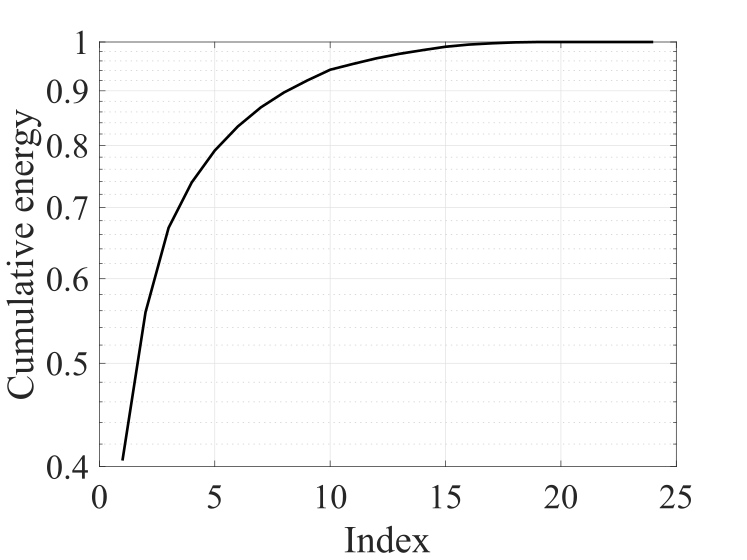
PCA was performed on the data matrix formed using 24 random flowfields chosen from the repository of 32 Pareto optimal solutions. The cumulative sum of the singular values, as well as the singular values themselves, show that within the first few PCA modes, significant energy or variance is captured by the principal components. As such, it is hoped that the first three principal components will be enough to represent the high-dimensional data and extract useful information.

The above figure shows all 24 cases in terms of their first three principal components. It demonstrates a clear dissociation between the solutions within each group, i.e., there is a tendency to form clusters. In other words, the unique flowfield characteristics that were seen earlier in the higher-dimensional data within each group of solutions (i.e., diffused compression waves and a strong oblique shock), is also retained in a lower dimensional space spanned by just three principal components. This goes on to show that such approaches can be used for image (or flowfield) classification when it might be difficult to do so for the raw data.

This analysis is part of a study undertaken in the Department of Aeronautics & Astronautics, Kyushu University, in collaboration with Mr. Ananthakrishnan Bhagyarajan (Post graduate student, UCLA) and Dr. Hideaki Ogawa (Associate Prof., Kyushu University).

Useful References: